This page explains how convolution interpolation works, where its accuracy comes from, and how convinterp’s kernels are defined. Every kernel is derived from its defining conditions in the code cells below, in exact rational arithmetic, whenever this documentation is built, and compared with the kernels convinterp evaluates.
Convolution interpolation
Given samples f_j = f(x_j) at uniformly spaced knots x_j = x_0 + jh, a convolution interpolant is a sum of shifted copies of one kernel function k, weighted by coefficients c_j:
Inside the data, the coefficients are the samples themselves, c_j = f_j. Near the ends, the sum also needs coefficients beyond the last knot; these are extrapolated from the data (see Boundaries). With x = x_0 + (i + t)h, 0 \le t < 1, only the knots within the kernel’s support contribute, so each evaluation is a short, fixed-length sum.
The kernels are piecewise polynomials: on each unit interval [i, i + 1], i = 0, \dots, M - 1, k is a polynomial P_i of degree p, it is even, k(-s) = k(s), and it vanishes for |s| \ge M. Each evaluation therefore combines 2M coefficients per axis, the kernel’s stencil.
Conditions on a kernel
Following Keys (1981), a kernel is defined by conditions on its polynomial pieces; Meijering et al. (1999) studied kernels of this kind systematically for higher polynomial degrees.
Interpolation.k(0) = 1 and k(i) = 0 at every other integer, so that \hat f(x_j) = f_j: the interpolant passes through the data.
Symmetry.k is even, so its odd derivatives vanish at s = 0.
Continuity. The derivatives of order 1, \dots, d are continuous at every knot, and vanish at the end of the support, s = M. The interpolant is then C^d.
Polynomial reproduction. For m = 0, \dots, R and all t,
\sum_j k(t - j)\, j^m = t^m.
\tag{2}
The last condition determines the accuracy. If it holds up to degree R, interpolating samples of any polynomial of degree \le R returns that polynomial exactly. For a smooth function, expanding each sample f(x_j) in a Taylor series around x shows that all terms up to order R are reproduced exactly, and the first term that is not has size h^{R+1}:
A kernel that reproduces polynomials up to degree R therefore converges at order R + 1. All four conditions are linear in the unknown polynomial coefficients, so a kernel is the solution of a linear system. Condition 4 is imposed as an identity in t: on 0 \le t < 1, both sides of Equation 2 are polynomials in t, and every coefficient must match.
Deriving a kernel
The module convinterp.derivation sets up this system and solves it exactly with SymPy (pip install convinterp[derivation]). With two pieces of degree 3, continuity C^1 and reproduction up to degree 2, the solution is unique: it is Keys’ cubic convolution kernel.
from convinterp.derivation import derive_kernel # the exact derivationkeys = derive_kernel(pieces=2, degree=3, continuity=1, reproduce=2) # Keys (1981)for i, piece inenumerate(keys): # one polynomial per unit interval terms = [f"({c}) s^{j}"for j, c inenumerate(piece) if c !=0] # nonzero terms, lowest power firstprint(f"on [{i}, {i +1}]: "+" + ".join(terms))
That is k(s) = 1 - \tfrac{5}{2}s^2 + \tfrac{3}{2}s^3 on [0, 1] and 2 - 4s + \tfrac{5}{2}s^2 - \tfrac{1}{2}s^3 on [1, 2], the kernel convinterp calls "a3". It reproduces quadratics, so it converges at 3rd order. With a third piece, the same conditions reach reproduction of cubics: Keys’ 4th-order kernel, "a4".
The b-series kernels
The b-series extends this construction to higher degrees and more pieces. For odd degree p \ge 5, the conditions
M = \frac{p + 5}{2}\ \text{pieces}, \qquad \text{continuity } C^{p-2}, \qquad
\text{reproduction up to degree } R = \min(p, 6)
\tag{4}
have exactly one solution, for every odd degree from 5 to 15 (verified exactly). The kernels "b5" to "b13" are these solutions. They were first found by a long exploratory search with symbolic computation, which combined the conditions above with additional fixed coefficients and a frequency-response criterion; the search script is kept in the Julia package ConvolutionInterpolations.jl. The direct formulation shows that no search is needed: the conditions alone determine each kernel, and it can be derived in seconds.
The cell below derives all of convinterp’s kernels, checks their continuity and polynomial reproduction exactly with kernel_properties, and compares each one with the kernel convinterp evaluates. For that comparison, it interpolates a unit impulse: data that are 1 at one knot and 0 at all others. By Equation 1, the interpolant of an impulse is the kernel itself.
import time # to time each derivationimport numpy as np # arraysfrom convinterp import convolution_interpolation # the compiled kernelsfrom convinterp.derivation import KERNEL_SETTINGS, kernel_properties, kernel_functionknots = np.arange(-15.0, 16.0) # integers, wide enough for every kernelimpulse = (knots ==0.0).astype(float) # 1 at the centre, 0 elsewhereprint("| Kernel | Pieces $M$ | Degree $p$ | Continuity | Reproduces up to | Order | ""Derivation time | Max. difference from compiled kernel |")print("|---|---|---|---|---|---|---|---|")derived = {}for name, settings in KERNEL_SETTINGS.items(): start = time.perf_counter() kernel = derive_kernel(*settings) # the unique solution seconds = time.perf_counter() - start derived[name] = kernel props = kernel_properties(kernel) # checked exactly, not assumed s = np.linspace(-props["pieces"] -0.5, props["pieces"] +0.5, 4001) compiled = convolution_interpolation(knots, impulse, kernel=name, bc="poly") difference = np.max(np.abs(compiled(s) - kernel_function(kernel)(s)))print(f'| `"{name}"` | {props["pieces"]} | {props["degree"]} | $C^{{{props["continuity"]}}}$ | 'f'{props["reproduces"]} | {props["reproduces"] +1} | {seconds:.1f} s | {difference:.1e} |')
Kernel
Pieces M
Degree p
Continuity
Reproduces up to
Order
Derivation time
Max. difference from compiled kernel
"a3"
2
3
C^{1}
2
3
0.0 s
2.6e-15
"a4"
3
3
C^{1}
3
4
0.0 s
2.6e-15
"b5"
5
5
C^{3}
5
6
0.4 s
2.6e-15
"b7"
6
7
C^{5}
6
7
1.0 s
2.6e-15
"b9"
7
9
C^{7}
6
7
2.2 s
2.6e-15
"b11"
8
11
C^{9}
6
7
4.3 s
2.6e-15
"b13"
9
13
C^{11}
6
7
7.4 s
2.6e-15
The differences are at the level of rounding: the compiled kernels are the derived ones. The reproduction degree also explains the orders of accuracy. "b5", with degree 5, can reproduce polynomials only up to degree 5 and converges at 6th order; from "b7" on, the kernels reach the design target of degree 6 and converge at 7th order. Higher degrees then add smoothness, not accuracy.
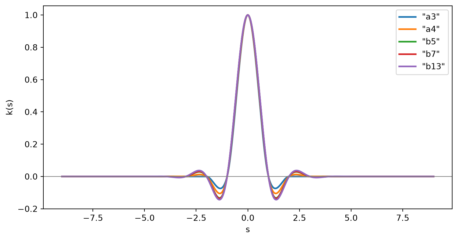
Figure 1 shows the kernels. All have the same basic shape, a central peak with small negative side lobes, like a truncated sinc function, and the wider kernels decay more gradually.
import matplotlib.pyplot as plt # plottings = np.linspace(-9.0, 9.0, 3601) # the widest support, b13fig, ax = plt.subplots(figsize=(9, 4.5))for name in ["a3", "a4", "b5", "b7", "b13"]: ax.plot(s, kernel_function(derived[name])(s), lw=2, label=f'"{name}"')ax.axhline(0.0, color="gray", lw=0.8) # the zero lineax.set_xlabel("s")ax.set_ylabel("k(s)")ax.legend()plt.show()
Figure 1: Kernels derived from their defining conditions. Each is 1 at s = 0 and 0 at every other integer.
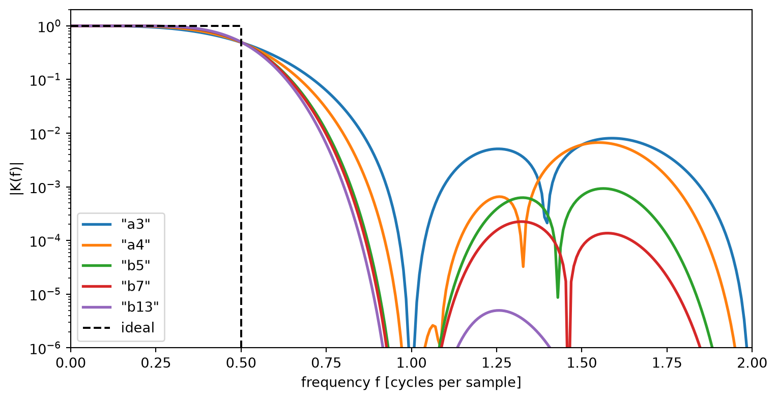
Figure 2 shows what the side lobes achieve. The Fourier transform of a kernel describes how the interpolant treats each frequency in the data. The ideal, the sinc function, passes every frequency below half the sampling rate unchanged and removes every frequency above it. All kernels pass the low frequencies almost unchanged; they differ in how well they suppress the high ones. Beyond one cycle per sample, Keys’ cubic lets through up to about 10^{-2} of the signal, "b7" about 2 \cdot 10^{-4}, and "b13" less than 10^{-5}.
def frequency_response(kernel, samples_per_unit=64, length=64):# |K(f)| by a fast Fourier transform of the kernel sampled finely over a long interval s = np.arange(-length, length, 1.0/ samples_per_unit) # fine samples, far beyond the support values = kernel_function(kernel)(s) spectrum = np.abs(np.fft.rfft(values)) / samples_per_unit # approximates the continuous transform f = np.fft.rfftfreq(len(s), d=1.0/ samples_per_unit) # frequencies in cycles per unit of sreturn f, spectrumfig, ax = plt.subplots(figsize=(9, 4.5))for name in ["a3", "a4", "b5", "b7", "b13"]: f, response = frequency_response(derived[name]) ax.plot(f, response, lw=2, label=f'"{name}"')ax.plot([0.0, 0.5, 0.5, 2.0], [1.0, 1.0, 0.0, 0.0], "k--", lw=1.5, label="ideal")ax.set_xlim(0.0, 2.0)ax.set_ylim(1e-6, 2.0)ax.set_yscale("log")ax.set_xlabel("frequency f [cycles per sample]")ax.set_ylabel("|K(f)|")ax.legend(loc="lower left")plt.show()
Figure 2: Frequency response |K(f)| of the kernels, with f in cycles per sample. The ideal interpolator passes everything below f = 0.5 and nothing above.
Boundaries
Near the ends of the data, Equation 1 needs coefficients c_j at up to M - 1 positions beyond the last knot. convinterp extrapolates them from the data, as ConvolutionInterpolations.jl does, and the boundary condition chooses how.
With bc="poly", the ghost values are polynomial extrapolation: at the left end, the value j steps beyond the first knot is
c_{-j} = \sum_{i=0}^{n-1} L_i(-j)\, f_i,
where L_i are the Lagrange basis polynomials of the n knots nearest the boundary (n = 4 for the a-series, 6 for "b5" and 8 from "b7" on). This extrapolation is exact for polynomials of degree up to n - 1, which is at least the kernel’s reproduction degree R. The interpolant therefore still reproduces polynomials of degree R right up to the boundary, and keeps its order of accuracy there. The weights L_i(-j) are integers, so they are exact in any floating-point precision.
Extrapolation of high degree amplifies whatever is in the data near the boundary. With bc="detect", the default, convinterp first checks whether the data there are smooth enough: it compares the n-th differences of the values near the boundary with their range, and falls back to linear extrapolation where the differences are too large. The user guide shows an example.
The extrapolation sums have large alternating weights: for the farthest ghost value of "b13", their magnitudes add up to about 10^6. convinterp therefore computes them with a compensated dot product (Ogita et al. 2005), as accurate as if computed in twice the working precision and then rounded. In more dimensions, the axes are extended one after the other, and the corner values are extrapolated again from ghost values; the compensated sums keep them as accurate as this construction allows.
Integrals
Because the interpolant is a finite sum of shifted kernels, it can be integrated term by term. Write x = x_0 + uh, with x_0 the first knot and x_j = x_0 + jh (negative j for the ghost values). The integral from the first knot is
\int_{x_0}^{x} \hat f(\xi)\, d\xi = h \sum_j c_j \bigl[K_1(u - j) - K_1(-j)\bigr],
\qquad K_1(s) = \int_0^s k(\sigma)\, d\sigma .
\tag{5}
K_1 is a piecewise polynomial of one degree higher than k, derived exactly from the kernel’s pieces. Reproducing constants, condition 4 with m = 0, implies \int k = 1, so outside the support K_1 is constant: K_1(s) = \pm\tfrac12 for \pm s \ge M. The coefficients in Equation 5 therefore fall into three groups:
Right of the stencil (j \ge u + M): the bracket is -\tfrac12 - (-\tfrac12) = 0. These coefficients don’t contribute.
In the stencil: the bracket is a polynomial in the position t within the cell, as for interpolation.
Left of the stencil (j \le u - M): the bracket no longer depends on t; it is 1 for coefficients far from the first knot, and an exact constant for the few near it.
The left group depends only on the cell the point lies in, so its sum is computed once for every cell, as a running sum over the coefficients, when the interpolant is created. Each evaluation then costs about as much as the interpolant itself, however many knots lie to the left.
Integrals of higher order m, all anchored at the first knot, follow in the same way. The kernel is replaced by its m-fold antiderivative K_m, minus the Taylor polynomial of degree m - 1 that makes the integral and all lower integrals vanish at x_0. Well left of the stencil, the weight of a coefficient becomes (u - j)^{m-1}/(m-1)!, which is Cauchy’s formula for repeated integration; it is a polynomial in t of degree m - 1. The left group is then a polynomial in t whose m coefficients are precomputed for every cell, again by running sums.
Integration does not cost accuracy: the error of the integral is the integral of the interpolation error, so it converges at least at the interpolant’s order. In more dimensions the kernel weights of the axes multiply, and with integrals along n axes the sum splits into 2^n parts, according to which integral axes have their coefficients left of the stencil. Each part is precomputed in the same way; together they take \prod_d (1 + m_d) - 1 times the memory of the data.
References
Keys, Robert G. 1981. “Cubic Convolution Interpolation for Digital Image Processing.”IEEE Transactions on Acoustics, Speech, and Signal Processing 29 (6): 1153–60. https://doi.org/10.1109/TASSP.1981.1163711.
Meijering, Erik H. W., Karel J. Zuiderveld, and Max A. Viergever. 1999. “Image Reconstruction by Convolution with Symmetrical Piecewise Nth-Order Polynomial Kernels.”IEEE Transactions on Image Processing 8 (2): 192–201. https://doi.org/10.1109/83.743854.
Ogita, Takeshi, Siegfried M. Rump, and Shin’ichi Oishi. 2005. “Accurate Sum and Dot Product.”SIAM Journal on Scientific Computing 26 (6): 1955–88. https://doi.org/10.1137/030601818.