User guide

convinterp has one function, convolution_interpolation. It takes data on a uniform grid and returns an interpolant: an object you call like a function, at any point inside the data range. This page walks through its arguments.

import numpy as np                                     # arrays
import matplotlib.pyplot as plt                        # plotting
from convinterp import convolution_interpolation       # the one function you need

Interpolating 1D data

The data are values at uniformly spaced, increasing knots:

x = np.linspace(0.0, 2 * np.pi, 40)                    # 40 uniformly spaced knots
y = np.sin(x)                                          # the data at the knots
itp = convolution_interpolation(x, y)                  # the interpolant, with the default kernel "b7"

Call it with a number to get a number, or with an array of any shape to get an array of the same shape:

print(itp(1.0))                                        # one point: a Python float
print(itp(np.array([0.5, 1.0, 1.5])))                  # several points: an array
print(itp(np.linspace(0.2, 1.2, 6).reshape(2, 3)))     # any shape is kept

0.8414709842567816
[0.47942554 0.84147098 0.99749499]
[[0.19866933 0.38941834 0.56464247]
 [0.71735609 0.84147098 0.93203909]]

The knots must be uniformly spaced (to a relative tolerance of 10^{-8} of the spacing), and points must lie inside the data range; anything else raises a ValueError that says what is wrong. Extrapolation beyond the data is not supported.

Choosing a kernel

The kernel argument selects the interpolation kernel. All kernels are piecewise polynomials that pass exactly through the data; they differ in accuracy, smoothness, how many derivatives and integrals they provide, and cost.

Kernel	Degree	Continuity	Derivatives up to	Integrals up to	Convergence	Stencil in N dimensions
`"a0"`	0	—	—	2	1st order	2^N
`"a1"`	1	C^0	—	2	2nd order	2^N
`"a3"`	3	C^1	1	4	3rd order	4^N
`"a4"`	3	C^1	1	4	4th order	6^N
`"a5"`	5	C^3	1	4	3rd order	6^N
`"a7"`	7	C^5	1	4	3rd order	8^N
`"b5"`	5	C^3	3	6	6th order	10^N
`"b7"`	7	C^5	5	8	7th order	12^N
`"b9"`	9	C^7	6	8	7th order	14^N
`"b11"`	11	C^9	7	8	7th order	16^N
`"b13"`	13	C^{11}	7	8	7th order	18^N

“Continuity” is how many derivatives of the interpolant are continuous, and “Stencil” is how many data values each evaluated point combines. The stencil sets the cost: in 3D, "b7" combines 12^3 = 1728 values per point. Continuity and convergence order follow exactly from the kernels’ rational coefficients: a kernel that reproduces polynomials up to degree m converges at order m + 1.

Some guidance:

"b7" is the default in 1D and 2D, and the right choice for most smooth data: 7th-order accuracy, five continuous derivatives.
"b7" to "b13" all converge at 7th order. The wider ones don’t interpolate more accurately; they are smoother and provide higher derivatives. Choose "b9" to "b13" when you need those.
"b5" converges at 6th order with a smaller stencil, which makes it the default in 3D. On coarse grids it behaves almost like the 7th-order kernels.
"a4" is a fast 4th-order kernel, comparable in accuracy to a cubic spline, and "a1" is linear interpolation. "a5" and "a7" are smoother than "a3" but converge at the same 3rd order.
kernel="auto" (the default) chooses by the number of dimensions, to keep the stencil affordable: "b7" for up to 2D, "b5" in 3D, "a4" in 4D and 5D, and "a3" beyond.

See Accuracy and performance for how the kernels compare in practice.

Derivatives

The derivative argument gives an interpolant of a derivative instead of the data. It is computed analytically from the kernel’s polynomial pieces, not by finite differences:

d1 = convolution_interpolation(x, y, derivative=1)     # the first derivative of the interpolant
d2 = convolution_interpolation(x, y, derivative=2)     # the second derivative
print(f"d1(1.0) = {d1(1.0):.10f},  cos(1.0)  = {np.cos(1.0):.10f}")
print(f"d2(1.0) = {d2(1.0):.10f},  -sin(1.0) = {-np.sin(1.0):.10f}")

d1(1.0) = 0.5403022965,  cos(1.0)  = 0.5403023059
d2(1.0) = -0.8414703517,  -sin(1.0) = -0.8414709848

Each kernel supports derivatives up to the order in the table above; asking for more raises a ValueError. Each derivative order costs about one order of convergence, as the derivative study shows.

Integrals

A negative derivative order gives an interpolant of an integral: derivative=-1 is the antiderivative, derivative=-2 the twofold integral, and so on. Integrals are anchored at the first knot: there the integral is zero, and so are all lower integrals. So derivative=-1 evaluated at b is \int_{x_0}^{b} of the interpolant. Like derivatives, integrals are computed analytically from the kernel’s polynomial pieces, not by numerical quadrature:

i1 = convolution_interpolation(x, y, derivative=-1)    # the integral from x[0] = 0
i2 = convolution_interpolation(x, y, derivative=-2)    # the twofold integral, also anchored at 0
print(f"i1(1.0) = {i1(1.0):.10f},  1 - cos(1.0) = {1 - np.cos(1.0):.10f}")
print(f"i2(1.0) = {i2(1.0):.10f},  1 - sin(1.0) = {1 - np.sin(1.0):.10f}")

i1(1.0) = 0.4596976943,  1 - cos(1.0) = 0.4596976941
i2(1.0) = 0.1585290154,  1 - sin(1.0) = 0.1585290152

A definite integral between two limits is the difference of two evaluations:

a, b = 1.0, 2.5                                        # the integration limits
integral = i1(b) - i1(a)                               # the integral of the interpolant from a to b
print(f"integral = {integral:.10f},  cos(a) - cos(b) = {np.cos(a) - np.cos(b):.10f}")

integral = 1.3414459212,  cos(a) - cos(b) = 1.3414459214

Integrals don’t cost convergence order: the integral of the interpolant is at least as accurate as the interpolant itself. Evaluating one costs about the same as the interpolant, whatever the number of knots, because the contribution of all data left of a point is precomputed when the interpolant is created. Each kernel supports integrals up to the order in the table above.

Boundary conditions

Near the ends of the data, a kernel’s stencil reaches beyond the last knot. convinterp fills those positions with extrapolated values, and the bc argument chooses how:

"poly": polynomial extrapolation of the degree the kernel reproduces. This keeps the full order of accuracy up to the boundary, for smooth data.
"linear" and "quadratic": lower-order extrapolation, robust for data that are not smooth near the boundary.
"detect" (the default): uses "poly" where the data near the boundary allow it, and falls back to "linear" where they don’t, decided separately at each boundary.

Figure 1 shows why the choice matters: data with a sharp step close to the right end. The polynomial extrapolation continues the step’s steepness beyond the data and makes the interpolant overshoot between the last knots; "detect" recognizes that the data there are not smooth and switches to linear extrapolation.

xs = np.linspace(0.0, 1.0, 21)                         # 21 knots on [0, 1]
ys = np.sin(3.0 * xs) + np.where(xs > 0.83, 1.0, 0.0)  # smooth data with a step near the right end
t = np.linspace(0.5, 1.0, 801)                         # fine points on the right half

fig, ax = plt.subplots(figsize=(9, 4.5))
for bc, style in [("poly", "-"), ("linear", "-"), ("detect", "--")]:
    itp_bc = convolution_interpolation(xs, ys, bc=bc)  # the same data, three boundary conditions
    ax.plot(t, itp_bc(t), style, lw=2.5 if bc == "detect" else 1.5, label=f'bc="{bc}"')
ax.plot(xs, ys, "ko", label="data")                    # the knots themselves
ax.set_xlim(0.5, 1.0)
ax.set_xlabel("x")
ax.legend(loc="upper left")
plt.show()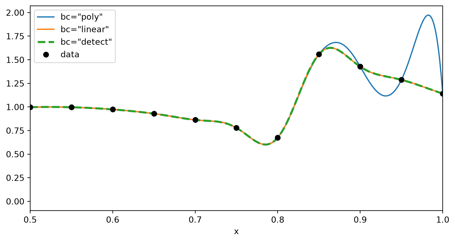

Figure 1: Interpolating data with a step near the right boundary. Polynomial extrapolation (“poly”) overshoots between the last knots; “detect” falls back to linear extrapolation there and stays close to the data.

The boundary condition can also be given per side, as a (left, right) pair, and in more dimensions per axis (see below):

itp = convolution_interpolation(x, y, bc=("poly", "linear"))  # polynomial on the left, linear on the right

Data in more dimensions

For data on an N-dimensional grid, give one knot array per axis, as a tuple. Axis d of the data array runs along knots[d], so a table data[i, j] belongs to the point (x[i], y[j]). With NumPy, np.meshgrid(x, y, indexing="ij") builds coordinates in this order.

xg = np.linspace(-1.0, 1.0, 12)                        # 12 knots along x
yg = np.linspace(-1.0, 1.0, 10)                        # 10 knots along y
X, Y = np.meshgrid(xg, yg, indexing="ij")              # coordinates, shape (12, 10)
field = np.exp(-2.0 * (X**2 + Y**2)) * np.cos(3.0 * X) # the data on the coarse grid
itp2 = convolution_interpolation((xg, yg), field)      # the 2D interpolant

Call it with one coordinate per axis. The coordinates are broadcast against each other like NumPy arrays, so a column of x values and a row of y values evaluate the whole table of combinations, as in Figure 2:

xf = np.linspace(-1.0, 1.0, 300)                       # fine x values
yf = np.linspace(-1.0, 1.0, 300)                       # fine y values
fine = itp2(xf[:, None], yf[None, :])                  # a column against a row: shape (300, 300)

fig, (ax1, ax2) = plt.subplots(1, 2, figsize=(10, 4.5))
extent = (-1.0, 1.0, -1.0, 1.0)                        # the plotted range, x then y
ax1.imshow(field.T, origin="lower", extent=extent, cmap="viridis")   # .T: imshow puts y vertically
ax1.set_title("data, 12 × 10")
ax2.imshow(fine.T, origin="lower", extent=extent, cmap="viridis")
ax2.set_title("interpolant, 300 × 300")
for ax in (ax1, ax2):
    ax.set_xlabel("x")
    ax.set_ylabel("y")
plt.show()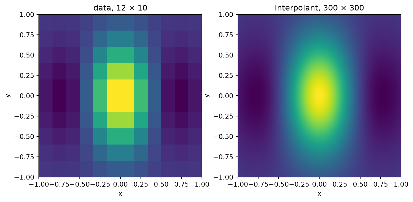

Figure 2: Left: data on a coarse 12 × 10 grid. Right: the 2D interpolant, evaluated on a 300 × 300 grid by broadcasting a column of x values against a row of y values.

The other arguments extend in the same way:

derivative is one order for every axis, or one per axis: derivative=(1, 0) is \partial/\partial x, and derivative=(1, 1) is \partial^2/\partial x\,\partial y. Negative orders integrate along their axis, each anchored at that axis’s first knot: derivative=(-1, -1) is the double integral from (x_0, y_0), and derivative=(-1, 1) integrates along x and differentiates along y. Integrals in N-D precompute tables of \prod_d (1 + m_d) - 1 times the size of the data, over the integral orders m_d; if that would exceed 2 GiB, a ValueError says so.
bc is one name for every boundary, one (left, right) pair for every axis, or a sequence of pairs, one per axis.
kernel is one kernel for all axes.

dx = convolution_interpolation((xg, yg), field, derivative=(1, 0))    # ∂/∂x
dxy = convolution_interpolation((xg, yg), field, derivative=(1, 1))   # ∂²/∂x∂y
ixy = convolution_interpolation((xg, yg), field, derivative=(-1, -1)) # ∫∫ from (xg[0], yg[0])
bcs = convolution_interpolation((xg, yg), field, bc=[("poly", "poly"), ("detect", "linear")])
print(dx(0.2, 0.1), dxy(0.2, 0.1), ixy(0.2, 0.1), bcs(0.2, 0.1))

-2.133076281700455 0.8510677712170592 0.28585933929391577 0.7466208703005504

Limitations

The high orders assume smooth, well-resolved data. Where that doesn’t hold, the kernels behave like any high-order interpolation:

Features near the grid resolution are damped. Oscillations faster than about half the Nyquist frequency (fewer than about four knots per period) are attenuated, and close to the Nyquist frequency the high-order kernels are no more accurate than a cubic spline.
Jumps ring, and kinks aren’t sharpened. At a discontinuity the interpolant overshoots by about 11 %, much like a cubic spline, and at a kink the higher orders don’t help. Linear interpolation ("a1") doesn’t overshoot.
Monotonicity and positivity aren’t preserved. Between the knots, the interpolant of monotone or positive data can overshoot. Where these must hold, use "a1", or a shape-preserving method such as SciPy’s PchipInterpolator.
Noise isn’t removed. The interpolant passes through every data value, noise included, and derivatives amplify noise however high the order: for noisy measurements, smooth first.
Polynomial boundaries need enough data. "poly" and "detect" need at least 4 data values along an axis for "a3" to "a7", 6 for "b5", and 8 for "b7" to "b13". With fewer, the boundaries fall back to linear extrapolation, and the kernel’s full order isn’t reached there.
"detect" is a heuristic. It tests how smooth the data are near each boundary. It reliably falls back to linear for noisy or rough boundary data, but a single outlier at the very end can pass as smooth. When you know your data, choose bc explicitly.

Not available yet

convinterp is in alpha. The Julia package it ports also provides interpolation of scattered, non-uniform data, and extrapolation beyond the data range. Scattered data are planned next; until then, convinterp covers interpolation, derivatives and integrals inside the range of data on uniform grids.