Accuracy and performance

This page compares convinterp with the standard alternatives in SciPy and NumPy: first how accurately it reproduces a difficult function and its derivatives, then how fast it evaluates. All figures are computed from the current code whenever this documentation is built.

Interpolation accuracy

Runge’s function, f(x) = 1/(1 + 25x^2) on [-1, 1], is smooth but notoriously difficult for polynomial interpolation on uniform grids. Figure 1 shows the maximum error over 11001 test points as the number of uniformly spaced samples grows from 10 to 10000.

import numpy as np                                     # arrays and Chebyshev evaluation
import matplotlib.pyplot as plt                        # plotting
from scipy.fft import dct                              # fast cosine transform, for Chebyshev coefficients
from scipy.interpolate import CubicSpline              # cubic spline reference
from convinterp import convolution_interpolation       # the package under test


def runge(x):
    # Runge's function: smooth, but hard for polynomial interpolation on uniform grids
    return 1.0 / (1.0 + 25.0 * x**2)


def chebyshev_coefficients(f, n):
    # coefficients of the interpolant of f at the n Chebyshev points of the first kind,
    # by a type-II DCT (stable and O(n log n))
    j = np.arange(n)                                                 # node indices 0 … n−1
    nodes = np.cos(np.pi * (j + 0.5) / n)                            # Chebyshev points of the first kind
    coefs = dct(f(nodes), type=2) / n                                # c_k = (2/n) Σ_j f(x_j) cos(πk(j + ½)/n)
    coefs[0] /= 2                                                    # the constant term has half weight
    return coefs


def convergence_study():
    x_test = np.linspace(-1.0, 1.0, 11_001)                          # dense test points
    y_test = runge(x_test)                                           # exact values there
    ns = np.unique(np.logspace(1, 4, 100).astype(int))               # 10 … 10000 samples, log-spaced
    kernels = ["a4", "b5", "b7", "b9", "b11", "b13"]                 # the kernels compared

    errors = {k: [] for k in kernels}                                # max error per kernel, per n
    spline_errors = []                                               # max error of the cubic spline
    cheb_errors = []                                                 # max error of Chebyshev interpolation

    for n in ns:
        x = np.linspace(-1.0, 1.0, n)                                # uniform grid with n samples
        y = runge(x)                                                 # the data on it
        for k in kernels:
            itp = convolution_interpolation(x, y, kernel=k)          # default boundary condition "detect"
            errors[k].append(np.max(np.abs(itp(x_test) - y_test)))   # maximum absolute error
        spline = CubicSpline(x, y)                                   # not-a-knot cubic spline
        spline_errors.append(np.max(np.abs(spline(x_test) - y_test)))
        coefs = chebyshev_coefficients(runge, n)                     # its own n non-uniform points
        cheb_errors.append(np.max(np.abs(np.polynomial.chebyshev.chebval(x_test, coefs) - y_test)))

    fig, ax = plt.subplots(figsize=(10, 6.5))                        # one log-log axis
    ax.loglog(ns, spline_errors, lw=2.5, color="orange", label="Cubic spline (SciPy)")
    for k in kernels:
        ax.loglog(ns, errors[k], lw=2, label=f'"{k}"')               # one line per convinterp kernel
    ax.loglog(ns, cheb_errors, lw=2.5, color="blue", label="Chebyshev (non-uniform points)")
    ax.loglog(ns, 1e-5 * (100.0 / ns) ** 7, "k--", lw=2, label=r"$\mathcal{O}(h^7)$")  # reference slope
    ax.set_xlim(10, 1e4)
    ax.set_ylim(1e-16, 1e0)
    ax.set_xlabel("Number of sample points")
    ax.set_ylabel("Maximum absolute error")
    ax.grid(True, which="both", alpha=0.3)                           # light grid for reading slopes
    ax.legend(loc="lower left")
    fig.tight_layout()
    return fig


fig = convergence_study()
plt.show()

Figure 1: Maximum interpolation error for Runge’s function. The kernels “b7” to “b13” converge at 7th order and “b5” at 6th, down to about 1e-15; “a4” matches a cubic spline at 4th order. Chebyshev interpolation, shown for reference, requires its own non-uniform sample points.

The kernels "b7" to "b13" follow the dashed \mathcal{O}(h^7) line until they reach the limit of double-precision arithmetic: 10^{-14} at about 900–1300 samples, and the rounding floor of about 10^{-15} by about 1100–1900, the wider kernels first. "b5" converges at 6th order, which shows as a slightly higher curve that approaches the others at the floor. The kernel "a4" converges at 4th order, like the cubic spline. Chebyshev interpolation converges faster than any fixed order, but only because it chooses its own sample points, clustered towards the ends of the interval. On uniformly sampled data, such as measurements, simulations and images, it cannot be used; there, the realistic alternative is a spline.

Derivative accuracy

Figure 2 shows the same study for the first three derivatives, compared with the exact derivatives of Runge’s function. convinterp evaluates derivatives analytically from the kernels’ polynomial pieces; the boundary condition here is "poly".

def runge_derivative(x, k):
    # the exact k-th derivative of Runge's function, for k = 1, 2, 3
    s = 1.0 + 25.0 * x**2                                            # the denominator's base
    if k == 1:
        return -50.0 * x / s**2
    if k == 2:
        return 50.0 * (75.0 * x**2 - 1.0) / s**3
    if k == 3:
        return 15000.0 * x * (1.0 - 25.0 * x**2) / s**4
    raise ValueError("k must be 1, 2 or 3")


def derivative_study(orders=(1, 2, 3)):
    x_test = np.linspace(-1.0, 1.0, 11_001)                          # dense test points
    ns = np.unique(np.logspace(1, 4, 100).astype(int))               # 10 … 10000 samples, log-spaced
    kernels = ["b5", "b7", "b9", "b11", "b13"]                       # all support derivatives up to 3

    fig, axes = plt.subplots(len(orders), 1, figsize=(10, 6 * len(orders)))  # panels stacked vertically
    for ax, k in zip(axes, orders):
        exact = runge_derivative(x_test, k)                          # the exact k-th derivative
        errors = {kern: [] for kern in kernels}                      # max error per kernel, per n
        spline_errors, cheb_errors = [], []                          # the two references

        for n in ns:
            x = np.linspace(-1.0, 1.0, n)                            # uniform grid with n samples
            y = runge(x)                                             # the data on it
            for kern in kernels:
                d_itp = convolution_interpolation(x, y, kernel=kern, bc="poly", derivative=k)
                errors[kern].append(np.max(np.abs(d_itp(x_test) - exact)))
            spline = CubicSpline(x, y)                               # not-a-knot cubic spline
            spline_errors.append(np.max(np.abs(spline(x_test, nu=k) - exact)))  # its k-th derivative
            coefs = np.polynomial.chebyshev.chebder(chebyshev_coefficients(runge, n), m=k)  # differentiate k times
            cheb_errors.append(np.max(np.abs(np.polynomial.chebyshev.chebval(x_test, coefs) - exact)))

        ax.loglog(ns, spline_errors, lw=2.5, color="orange", label="Cubic spline (SciPy)")
        for kern in kernels:
            ax.loglog(ns, errors[kern], lw=2, label=f'"{kern}"')     # one line per convinterp kernel
        ax.loglog(ns, cheb_errors, lw=2.5, color="blue", label="Chebyshev")
        i100 = np.argmin(np.abs(ns - 100))                           # anchor the slope line near n = 100
        anchor = 10.0 * errors["b7"][i100]                           # a decade above the b7 curve there
        ax.loglog(ns, anchor * (ns[i100] / ns) ** (7 - k), "k--", lw=2,
                  label=rf"$\mathcal{{O}}(h^{{{7 - k}}})$")          # the expected order: 7 − k
        ax.set_xlim(10, 1e4)
        ax.set_title(rf"derivative order {k}")
        ax.set_xlabel("Number of sample points")
        ax.set_ylabel("Maximum absolute error")                      # every panel has its own scale
        ax.grid(True, which="both", alpha=0.3)                       # light grid for reading slopes
        ax.legend(loc="lower left")
    fig.tight_layout()
    return fig


fig = derivative_study()
plt.show()

Figure 2: Maximum error of the first three derivatives of Runge’s function. The b-series kernels lose one order of convergence per derivative (dashed lines for “b7” to “b13”), and their rounding floor rises slowly. Chebyshev differentiation converges fastest but amplifies rounding by about n² per derivative order.

Each derivative costs the b-series kernels one order of convergence: for "b7" to "b13", 6th order for the first derivative, 5th for the second and 4th for the third, and one order less for "b5". Their rounding floor rises slowly with the number of samples, roughly in proportion to n^k for the k-th derivative, which is unavoidable when differentiating sampled data. Chebyshev differentiation reaches its best accuracy with fewer samples, but its rounding grows about n^2 per derivative order: for the third derivative it becomes worse than no interpolation at all. The cubic spline converges at 4 - k for the k-th derivative, so its third derivative is piecewise constant.

Integral accuracy

Figure 3 shows the same study for the first three integrals, each anchored at x = -1: zero there, together with all lower integrals. convinterp evaluates integrals analytically from the kernels’ polynomial pieces; SciPy’s cubic spline and NumPy’s Chebyshev series are integrated with the same anchoring.

def runge_integral(x, k):
    # the exact k-th integral of Runge's function from −1, with all lower integrals zero there
    a5 = np.arctan(5.0)                                              # arctan(5), from the lower limit
    def G(s):
        # an antiderivative of arctan(5s)
        return s * np.arctan(5.0 * s) - np.log(1.0 + 25.0 * s**2) / 10.0
    def H(s):
        # an antiderivative of G
        return ((s**2 / 2.0) * np.arctan(5.0 * s) - s / 10.0 + np.arctan(5.0 * s) / 50.0
                - (s * np.log(1.0 + 25.0 * s**2) - 2.0 * s + 0.4 * np.arctan(5.0 * s)) / 10.0)
    if k == 1:
        return (np.arctan(5.0 * x) + a5) / 5.0
    if k == 2:
        return (G(x) - G(-1.0)) / 5.0 + a5 / 5.0 * (x + 1.0)
    if k == 3:
        return (H(x) - H(-1.0) - G(-1.0) * (x + 1.0)) / 5.0 + a5 / 5.0 * (x + 1.0)**2 / 2.0
    raise ValueError("k must be 1, 2 or 3")


def integral_study(orders=(1, 2, 3)):
    x_test = np.linspace(-1.0, 1.0, 11_001)                          # dense test points
    ns = np.unique(np.logspace(1, 4, 100).astype(int))               # 10 … 10000 samples, log-spaced
    kernels = ["b5", "b7", "b9", "b11", "b13"]                       # the high-order kernels

    fig, axes = plt.subplots(len(orders), 1, figsize=(10, 6 * len(orders)))  # panels stacked vertically
    for ax, k in zip(axes, orders):
        exact = runge_integral(x_test, k)                            # the exact k-th integral
        errors = {kern: [] for kern in kernels}                      # max error per kernel, per n
        spline_errors, cheb_errors = [], []                          # the two references

        for n in ns:
            x = np.linspace(-1.0, 1.0, n)                            # uniform grid with n samples
            y = runge(x)                                             # the data on it
            for kern in kernels:
                i_itp = convolution_interpolation(x, y, kernel=kern, bc="poly", derivative=-k)
                errors[kern].append(np.max(np.abs(i_itp(x_test) - exact)))
            spline = CubicSpline(x, y).antiderivative(k)             # k-th integral, zero at x = −1
            spline_errors.append(np.max(np.abs(spline(x_test) - exact)))
            coefs = np.polynomial.chebyshev.chebint(chebyshev_coefficients(runge, n), m=k, lbnd=-1.0)
            cheb_errors.append(np.max(np.abs(np.polynomial.chebyshev.chebval(x_test, coefs) - exact)))

        ax.loglog(ns, spline_errors, lw=2.5, color="orange", label="Cubic spline (SciPy)")
        for kern in kernels:
            ax.loglog(ns, errors[kern], lw=2, label=f'"{kern}"')     # one line per convinterp kernel
        ax.loglog(ns, cheb_errors, lw=2.5, color="blue", label="Chebyshev")
        i100 = np.argmin(np.abs(ns - 100))                           # anchor the slope line near n = 100
        anchor = 10.0 * errors["b7"][i100]                           # a decade above the b7 curve there
        ax.loglog(ns, anchor * (ns[i100] / ns) ** 7, "k--", lw=2,
                  label=r"$\mathcal{O}(h^{7})$")                     # the rate of "b7" to "b13"
        ax.set_xlim(10, 1e4)
        largest = max(max(spline_errors), max(cheb_errors), *(max(e) for e in errors.values()))
        ax.set_ylim(1e-17, 10.0 * largest)                           # from below the rounding floor to a decade above the largest error
        ax.set_title(rf"integral order {k}")
        ax.set_xlabel("Number of sample points")
        ax.set_ylabel("Maximum absolute error")                      # every panel has its own scale
        ax.grid(True, which="both", alpha=0.3)                       # light grid for reading slopes
        ax.legend(loc="lower left")
    fig.tight_layout()
    return fig


fig = integral_study()
plt.show()

Figure 3: Maximum error of the first three integrals of Runge’s function, anchored at x = −1. The b-series kernels converge at their interpolation order (dashed lines: 7th order, the rate of “b7” to “b13”), down to rounding; unlike for derivatives, their rounding floor stays low.

The integrals converge at the order of the interpolant: 7th for "b7" to "b13" (dashed lines) and 6th for "b5", since the error of an integral is the integral of the interpolation error. Integration doesn’t amplify rounding: unlike for derivatives, the error floor doesn’t rise with the number of samples.

Evaluation speed

Figure 4 compares the time per evaluated point with SciPy’s standard interpolators, in 1D and 2D, and for integrals in 1D. Every interpolant is built before the timing starts, and all points are evaluated in one vectorized call, taking the fastest of five runs.

import time                                            # wall-clock timing
from scipy.interpolate import make_interp_spline, RegularGridInterpolator, RectBivariateSpline


def ns_per_point(evaluate, n_points, repeats=5):
    # the best of `repeats` timings of one vectorized call, in nanoseconds per point
    best = np.inf                                                    # fastest run so far
    for _ in range(repeats):
        start = time.perf_counter()                                  # high-resolution clock
        evaluate()                                                   # evaluate at all points at once
        best = min(best, time.perf_counter() - start)                # keep the fastest run
    return 1e9 * best / n_points                                     # seconds per call → ns per point


def timing_1d(n_knots=1000, n_points=1_000_000):
    # evaluation time per point in 1D, at random (unsorted) points
    rng = np.random.default_rng(0)                                   # reproducible points
    x = np.linspace(0.0, 1.0, n_knots)                               # uniform grid
    y = np.sin(8.0 * x) + 0.3 * x                                    # smooth data on it
    p = rng.uniform(0.0, 1.0, n_points)                              # the evaluation points
    convinterp, scipy = {}, {}                                       # ns per point, by method
    for k in ["a1", "a3", "a4", "b5", "b7", "b9", "b11", "b13"]:
        itp = convolution_interpolation(x, y, kernel=k)              # built once, outside the timing
        convinterp[f'"{k}"'] = ns_per_point(lambda: itp(p), n_points)
    scipy["np.interp (linear)"] = ns_per_point(lambda: np.interp(p, x, y), n_points)
    spline = CubicSpline(x, y)                                       # cubic spline
    scipy["CubicSpline"] = ns_per_point(lambda: spline(p), n_points)
    for degree in (5, 7):
        bspline = make_interp_spline(x, y, k=degree)                 # interpolating B-spline
        scipy[f"B-spline, degree {degree}"] = ns_per_point(lambda: bspline(p), n_points)
    return convinterp, scipy


def timing_2d(n_knots=200, n_points=200_000):
    # evaluation time per point in 2D, at random points on a 200 × 200 grid
    rng = np.random.default_rng(1)                                   # reproducible points
    x = np.linspace(0.0, 1.0, n_knots)                               # knots of axis 0
    y = np.linspace(0.0, 1.0, n_knots)                               # knots of axis 1
    data = np.sin(8.0 * x)[:, None] * np.cos(5.0 * y)[None, :]       # smooth data on the grid
    px = rng.uniform(0.0, 1.0, n_points)                             # x coordinates of the points
    py = rng.uniform(0.0, 1.0, n_points)                             # y coordinates of the points
    pxy = np.column_stack([px, py])                                  # the same points as rows, for SciPy
    convinterp, scipy = {}, {}                                       # ns per point, by method
    for k in ["a1", "a3", "a4", "b5", "b7"]:
        itp = convolution_interpolation((x, y), data, kernel=k)      # built once, outside the timing
        convinterp[f'"{k}"'] = ns_per_point(lambda: itp(px, py), n_points)
    for method in ["linear", "cubic", "quintic"]:
        rgi = RegularGridInterpolator((x, y), data, method=method)   # SciPy's grid interpolator
        scipy[f"RegularGridInterpolator, {method}"] = ns_per_point(lambda: rgi(pxy), n_points)
    for degree in (3, 5):
        rbs = RectBivariateSpline(x, y, data, kx=degree, ky=degree)  # tensor-product spline
        scipy[f"RectBivariateSpline, degree {degree}"] = ns_per_point(
            lambda: rbs(px, py, grid=False), n_points)               # grid=False: evaluate point by point
    return convinterp, scipy


def timing_1d_integrals(n_knots=1000, n_points=1_000_000):
    # evaluation time per point of first integrals in 1D, at random (unsorted) points
    rng = np.random.default_rng(2)                                   # reproducible points
    x = np.linspace(0.0, 1.0, n_knots)                               # uniform grid
    y = np.sin(8.0 * x) + 0.3 * x                                    # smooth data on it
    p = rng.uniform(0.0, 1.0, n_points)                              # the evaluation points
    convinterp, scipy = {}, {}                                       # ns per point, by method
    for k in ["a1", "a3", "a4", "b5", "b7", "b9", "b11", "b13"]:
        itp = convolution_interpolation(x, y, kernel=k, derivative=-1)  # the integral from x[0]
        convinterp[f'"{k}"'] = ns_per_point(lambda: itp(p), n_points)
    spline = CubicSpline(x, y).antiderivative(1)                     # the spline's integral from x[0]
    scipy["CubicSpline, antiderivative"] = ns_per_point(lambda: spline(p), n_points)
    for degree in (5, 7):
        bspline = make_interp_spline(x, y, k=degree).antiderivative(1)  # the B-spline's integral
        scipy[f"B-spline, degree {degree}, antiderivative"] = ns_per_point(lambda: bspline(p), n_points)
    return convinterp, scipy


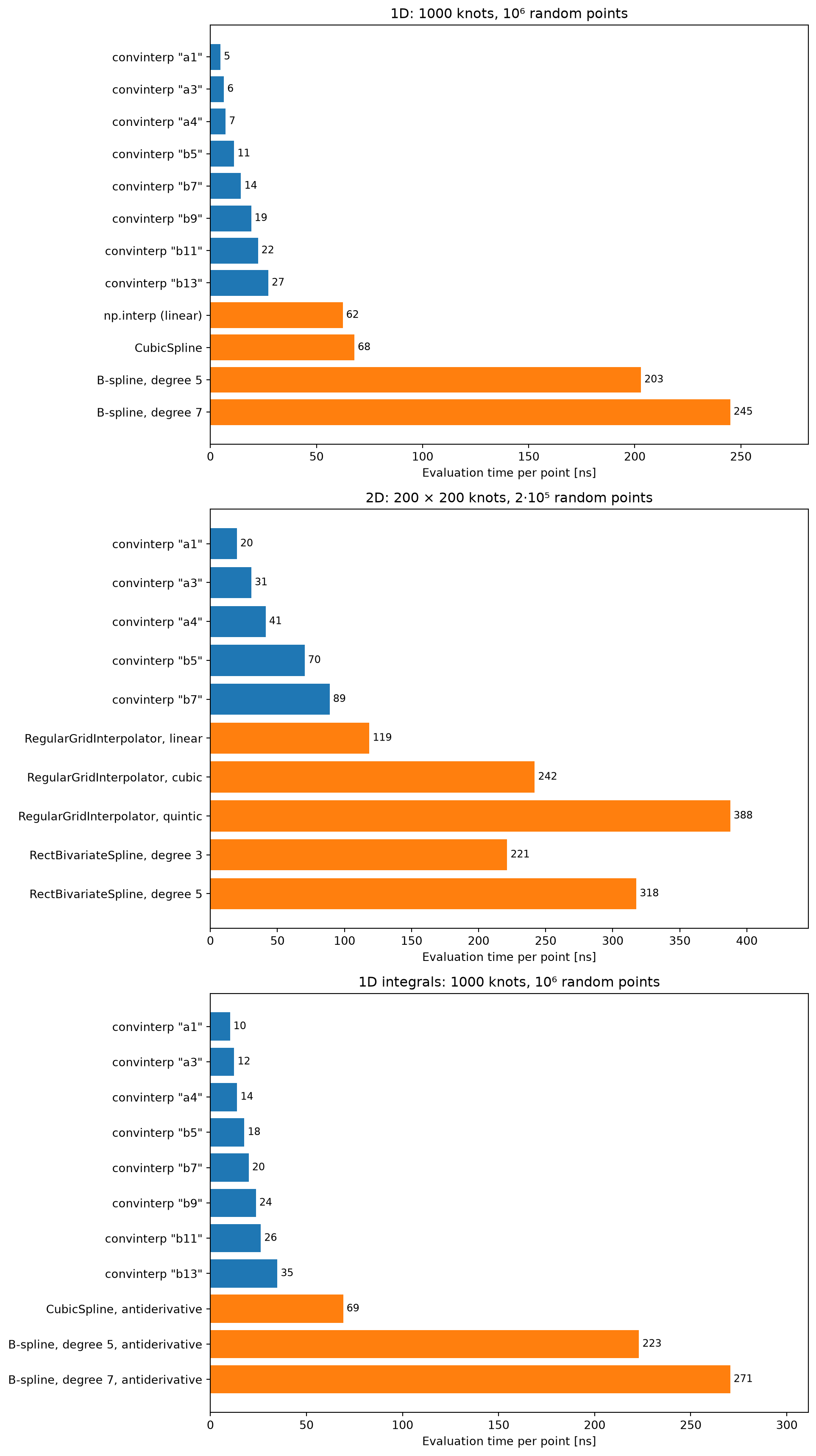
def bar_panel(ax, convinterp, scipy, title):
    # horizontal bars: convinterp kernels on top, SciPy methods below, with the times written out
    labels = [f"convinterp {k}" for k in convinterp] + list(scipy)   # one bar per method
    times = list(convinterp.values()) + list(scipy.values())         # ns per point, same order
    colors = ["tab:blue"] * len(convinterp) + ["tab:orange"] * len(scipy)
    rows = np.arange(len(labels))                                    # one row per bar
    ax.barh(rows, times, color=colors)
    ax.set_yticks(rows, labels)
    ax.invert_yaxis()                                                # first entry at the top
    for row, t in zip(rows, times):
        ax.text(t, row, f" {t:.0f}", va="center", fontsize=9)        # the time next to each bar
    ax.set_xlim(0, 1.15 * max(times))                                # room for the labels
    ax.set_xlabel("Evaluation time per point [ns]")
    ax.set_title(title)


def timing_figure():
    c1, s1 = timing_1d()                                             # 1D timings
    c2, s2 = timing_2d()                                             # 2D timings
    c3, s3 = timing_1d_integrals()                                   # 1D integral timings
    fig, (ax1, ax2, ax3) = plt.subplots(3, 1, figsize=(10, 18))      # 1D, 2D, integrals, stacked
    bar_panel(ax1, c1, s1, "1D: 1000 knots, 10⁶ random points")
    bar_panel(ax2, c2, s2, "2D: 200 × 200 knots, 2·10⁵ random points")
    bar_panel(ax3, c3, s3, "1D integrals: 1000 knots, 10⁶ random points")
    fig.tight_layout()
    return fig


fig = timing_figure()
plt.show()

Figure 4: Evaluation time per point, convinterp (blue) and SciPy (orange). Top: interpolation in 1D; middle: in 2D; bottom: first integrals in 1D, against the antiderivatives of SciPy’s splines. Measured on the machine that built this page, at build time: absolute times vary between machines, but the ratios between methods are what matters.

On a uniform grid, locating a point takes a single division, where SciPy’s general-purpose interpolators search the knots. The kernel weights are exact polynomials, evaluated for the whole stencil at once in compiled, vectorized Rust. As a result, even the widest kernel, "b13", evaluates faster than SciPy’s linear interpolation, and at comparable orders of accuracy the difference is several times: "a4" against the cubic spline, and the b-series kernels against the degree-5 and degree-7 splines.

Integrals cost about as much as the interpolant itself: the contribution of everything left of a point is precomputed when the interpolant is built, so each evaluation is one stencil sum plus a short polynomial, whatever the number of knots. SciPy’s antiderivatives are splines of one degree higher, evaluated like the originals, with the same search for each point.