The first three integrals of Runge’s function from uniformly spaced samples, each anchored at x = -1: convinterp’s analytic antiderivatives of its kernels, against the antiderivatives of SciPy’s cubic spline and of Chebyshev interpolation. Then the definite integral over the whole interval against SciPy’s quadrature rules on the samples, and the evaluation speed of the antiderivatives.
Packages and the test function
import numpy as np # arrays and Chebyshev evaluationimport matplotlib.pyplot as plt # plottingfrom scipy.fft import dct # fast cosine transform, for Chebyshev coefficientsfrom scipy.interpolate import CubicSpline # cubic spline referencefrom convinterp import convolution_interpolation # the package under testdef runge(x):# Runge's function: smooth, but hard for polynomial interpolation on uniform gridsreturn1.0/ (1.0+25.0* x**2)def runge_integral(x, k):# the exact k-th integral of Runge's function from −1, with all lower integrals zero there a5 = np.arctan(5.0) # arctan(5), from the lower limitdef G(s):# an antiderivative of arctan(5s)return s * np.arctan(5.0* s) - np.log(1.0+25.0* s**2) /10.0def H(s):# an antiderivative of Greturn ((s**2/2.0) * np.arctan(5.0* s) - s /10.0+ np.arctan(5.0* s) /50.0- (s * np.log(1.0+25.0* s**2) -2.0* s +0.4* np.arctan(5.0* s)) /10.0)if k ==1:return (np.arctan(5.0* x) + a5) /5.0if k ==2:return (G(x) - G(-1.0)) /5.0+ a5 /5.0* (x +1.0)if k ==3:return (H(x) - H(-1.0) - G(-1.0) * (x +1.0)) /5.0+ a5 /5.0* (x +1.0)**2/2.0raiseValueError("k must be 1, 2 or 3")def chebyshev_coefficients(f, n):# coefficients of the interpolant of f at the n Chebyshev points of the first kind,# by a type-II DCT (stable and O(n log n)) j = np.arange(n) # node indices 0 … n−1 nodes = np.cos(np.pi * (j +0.5) / n) # Chebyshev points of the first kind coefs = dct(f(nodes), type=2) / n # c_k = (2/n) Σ_j f(x_j) cos(πk(j + ½)/n) coefs[0] /=2# the constant term has half weightreturn coefs
Accuracy of the antiderivatives
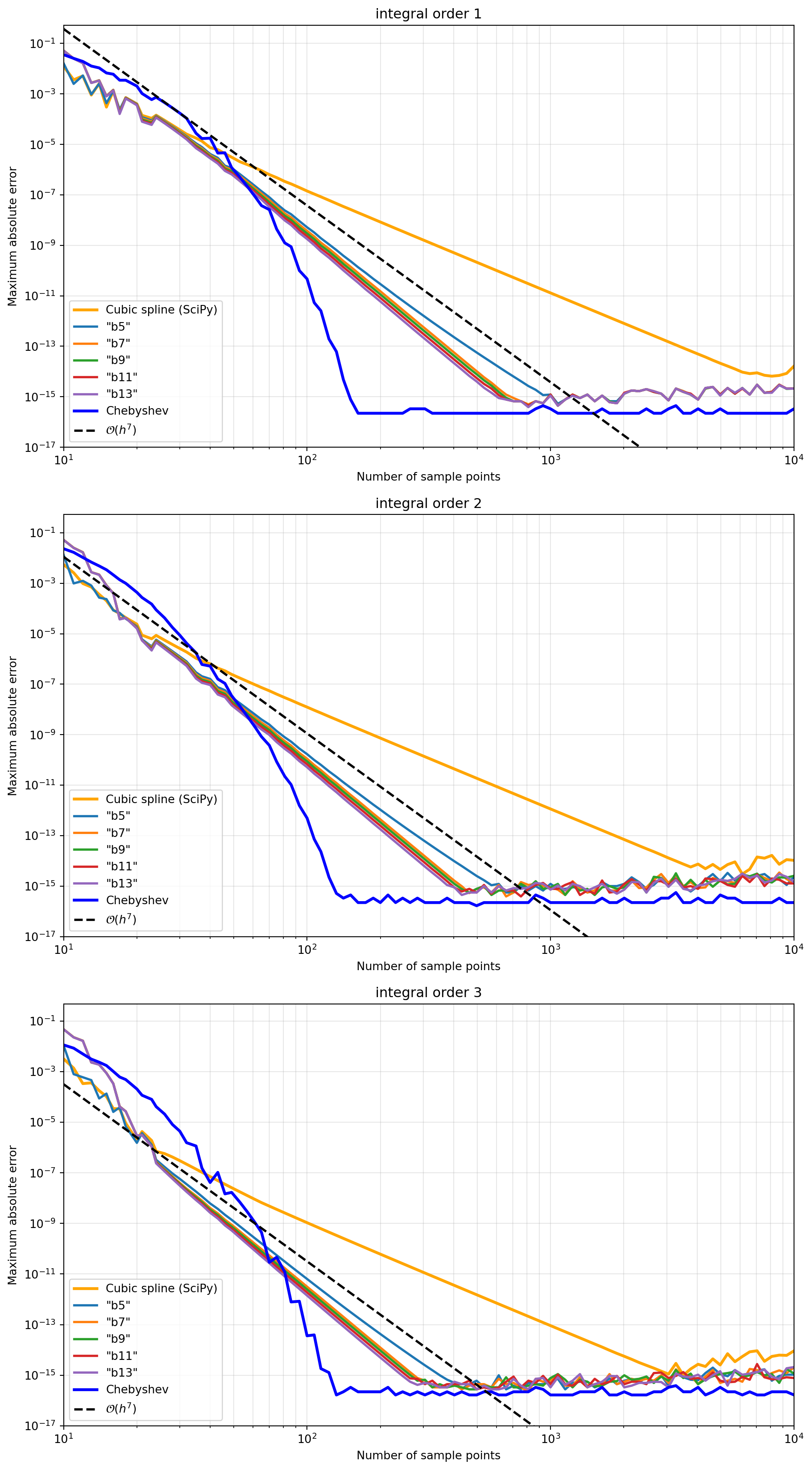
Figure 1 shows the maximum error of each integral over a dense set of test points as the number of samples grows. convinterp evaluates integrals analytically from the kernels’ polynomial pieces; SciPy’s cubic spline and NumPy’s Chebyshev series are integrated with the same anchoring.
Code
def integral_study(orders=(1, 2, 3)): x_test = np.linspace(-1.0, 1.0, 11_001) # dense test points ns = np.unique(np.logspace(1, 4, 100).astype(int)) # 10 … 10000 samples, log-spaced kernels = ["b5", "b7", "b9", "b11", "b13"] # the high-order kernels fig, axes = plt.subplots(len(orders), 1, figsize=(10, 6*len(orders))) # panels stacked verticallyfor ax, k inzip(axes, orders): exact = runge_integral(x_test, k) # the exact k-th integral errors = {kern: [] for kern in kernels} # max error per kernel, per n spline_errors, cheb_errors = [], [] # the two referencesfor n in ns: x = np.linspace(-1.0, 1.0, n) # uniform grid with n samples y = runge(x) # the data on itfor kern in kernels: i_itp = convolution_interpolation(x, y, kernel=kern, bc="poly", derivative=-k) errors[kern].append(np.max(np.abs(i_itp(x_test) - exact))) spline = CubicSpline(x, y).antiderivative(k) # k-th integral, zero at x = −1 spline_errors.append(np.max(np.abs(spline(x_test) - exact))) coefs = np.polynomial.chebyshev.chebint(chebyshev_coefficients(runge, n), m=k, lbnd=-1.0) cheb_errors.append(np.max(np.abs(np.polynomial.chebyshev.chebval(x_test, coefs) - exact))) ax.loglog(ns, spline_errors, lw=2.5, color="orange", label="Cubic spline (SciPy)")for kern in kernels: ax.loglog(ns, errors[kern], lw=2, label=f'"{kern}"') # one line per convinterp kernel ax.loglog(ns, cheb_errors, lw=2.5, color="blue", label="Chebyshev") i100 = np.argmin(np.abs(ns -100)) # anchor the slope line near n = 100 anchor =10.0* errors["b7"][i100] # a decade above the b7 curve there ax.loglog(ns, anchor * (ns[i100] / ns) **7, "k--", lw=2, label=r"$\mathcal{O}(h^{7})$") # the rate of "b7" to "b13" ax.set_xlim(10, 1e4) largest =max(max(spline_errors), max(cheb_errors), *(max(e) for e in errors.values())) ax.set_ylim(1e-17, 10.0* largest) # from below the rounding floor to a decade above the largest error ax.set_title(rf"integral order {k}") ax.set_xlabel("Number of sample points") ax.set_ylabel("Maximum absolute error") # every panel has its own scale ax.grid(True, which="both", alpha=0.3) # light grid for reading slopes ax.legend(loc="lower left") fig.tight_layout()return figfig = integral_study()plt.show()
Figure 1: Maximum error of the first three integrals of Runge’s function, anchored at x = −1. The b-series kernels converge at their interpolation order (dashed lines: 7th order, the rate of “b7” to “b13”), down to rounding; unlike for derivatives, their rounding floor stays low.
The integrals converge at the order of the interpolant: 7th for "b7" to "b13" (dashed lines) and 6th for "b5", since the error of an integral is the integral of the interpolation error. Integration doesn’t amplify rounding: unlike for derivatives, the error floor doesn’t rise with the number of samples.
Definite integrals against quadrature rules
The usual way to integrate sampled data is a quadrature rule on the samples. The integral of Runge’s function over the whole interval, from 2^k + 1 samples so that Romberg’s rule applies, as a relative error:
The quadrature comparison
from scipy.integrate import simpson, rombexact_total =2.0* np.arctan(5.0) /5.0# ∫ from −1 to 1 of Runge's functionrows = []for n in [9, 17, 33, 65, 129, 257, 513]: x = np.linspace(-1.0, 1.0, n) # 2^k + 1 uniform samples y = runge(x) h = x[1] - x[0] # the spacing, for Romberg i_b7 = convolution_interpolation(x, y, kernel="b7", bc="poly", derivative=-1) # the antiderivative rows.append((n,abs(simpson(y, x=x) - exact_total) / exact_total,abs(romb(y, dx=h) - exact_total) / exact_total,abs(CubicSpline(x, y).integrate(-1.0, 1.0) - exact_total) / exact_total,abs(i_b7(1.0) - exact_total) / exact_total))
samples
Simpson
Romberg
cubic spline
convinterp “b7”
9
4.7e-02
4.7e-02
1.2e-02
2.2e-01
17
4.9e-03
1.2e-03
1.1e-04
3.1e-05
33
3.3e-05
3.4e-04
3.3e-07
2.2e-08
65
1.7e-08
4.1e-06
1.1e-08
1.6e-11
129
9.5e-10
2.0e-08
4.4e-10
2.3e-14
257
5.9e-11
1.7e-10
2.1e-11
8.1e-16
513
3.7e-12
1.8e-13
1.1e-12
2.0e-16
The quadrature rules give one number for one interval; the antiderivative interpolant gives the integral to any point, and the difference of two evaluations gives the integral over any sub-interval, at the same accuracy.
Evaluation speed
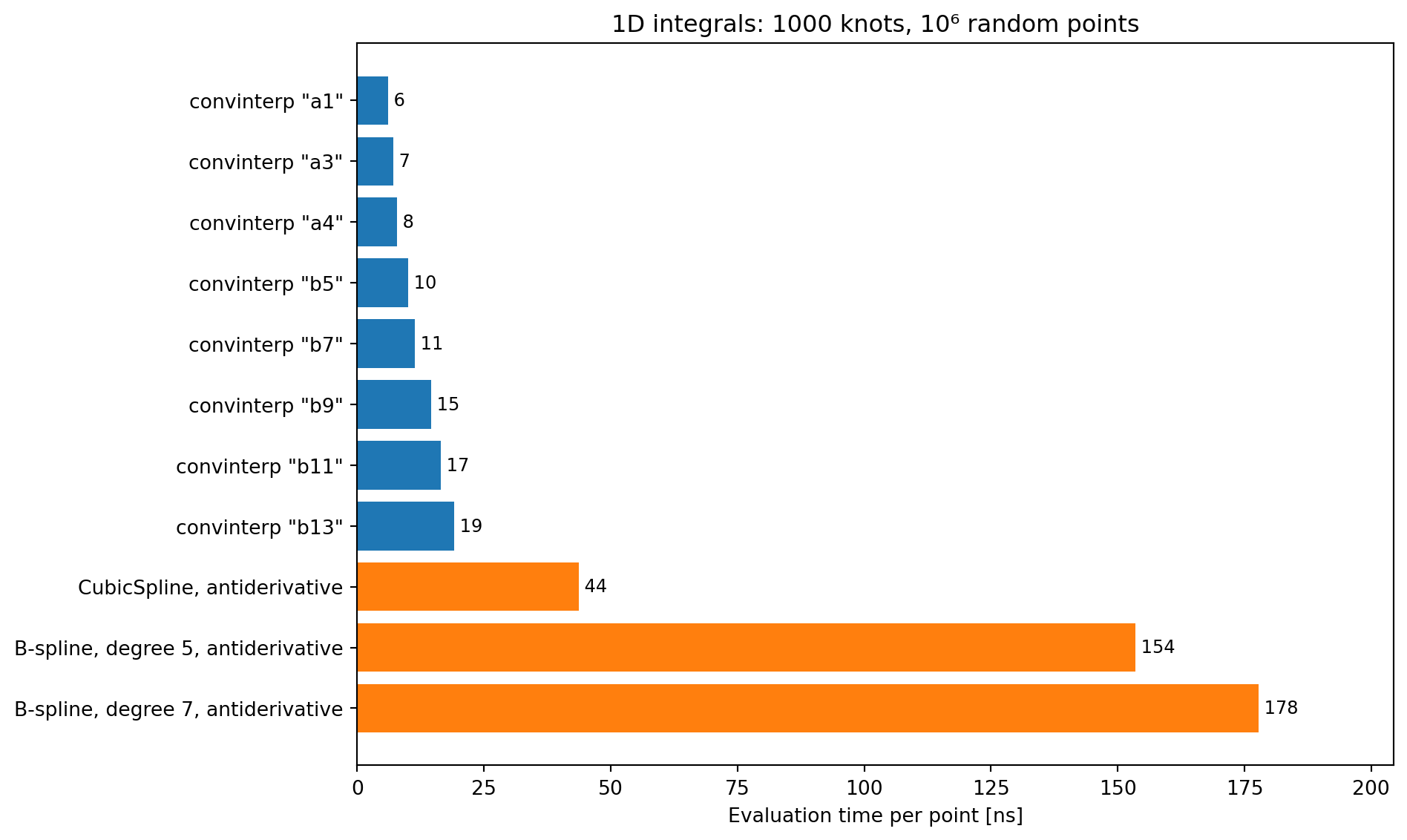
Figure 2 compares the time per evaluated point of first integrals in 1D, against the antiderivatives of SciPy’s splines. Every interpolant is built before the timing starts, and all points are evaluated in one vectorized call, taking the fastest of five runs.
Code
import time # wall-clock timingfrom scipy.interpolate import make_interp_splinedef ns_per_point(evaluate, n_points, repeats=5):# the best of `repeats` timings of one vectorized call, in nanoseconds per point best = np.inf # fastest run so farfor _ inrange(repeats): start = time.perf_counter() # high-resolution clock evaluate() # evaluate at all points at once best =min(best, time.perf_counter() - start) # keep the fastest runreturn1e9* best / n_points # seconds per call → ns per pointdef timing_1d_integrals(n_knots=1000, n_points=1_000_000):# evaluation time per point of first integrals in 1D, at random (unsorted) points rng = np.random.default_rng(2) # reproducible points x = np.linspace(0.0, 1.0, n_knots) # uniform grid y = np.sin(8.0* x) +0.3* x # smooth data on it p = rng.uniform(0.0, 1.0, n_points) # the evaluation points convinterp, scipy = {}, {} # ns per point, by methodfor k in ["a1", "a3", "a4", "b5", "b7", "b9", "b11", "b13"]: itp = convolution_interpolation(x, y, kernel=k, derivative=-1) # the integral from x[0] convinterp[f'"{k}"'] = ns_per_point(lambda: itp(p), n_points) spline = CubicSpline(x, y).antiderivative(1) # the spline's integral from x[0] scipy["CubicSpline, antiderivative"] = ns_per_point(lambda: spline(p), n_points)for degree in (5, 7): bspline = make_interp_spline(x, y, k=degree).antiderivative(1) # the B-spline's integral scipy[f"B-spline, degree {degree}, antiderivative"] = ns_per_point(lambda: bspline(p), n_points)return convinterp, scipydef bar_panel(ax, convinterp, scipy, title):# horizontal bars: convinterp kernels on top, SciPy methods below, with the times written out labels = [f"convinterp {k}"for k in convinterp] +list(scipy) # one bar per method times =list(convinterp.values()) +list(scipy.values()) # ns per point, same order colors = ["tab:blue"] *len(convinterp) + ["tab:orange"] *len(scipy) rows = np.arange(len(labels)) # one row per bar ax.barh(rows, times, color=colors) ax.set_yticks(rows, labels) ax.invert_yaxis() # first entry at the topfor row, t inzip(rows, times): ax.text(t, row, f" {t:.0f}", va="center", fontsize=9) # the time next to each bar ax.set_xlim(0, 1.15*max(times)) # room for the labels ax.set_xlabel("Evaluation time per point [ns]") ax.set_title(title)c3, s3 = timing_1d_integrals() # 1D integral timingsfig, ax = plt.subplots(figsize=(10, 6))bar_panel(ax, c3, s3, "1D integrals: 1000 knots, 10⁶ random points")fig.tight_layout()plt.show()
Figure 2: Evaluation time per point of first integrals in 1D, convinterp (blue) against the antiderivatives of SciPy’s splines (orange). Measured on the machine that built this page, at build time.
Integrals cost about as much as the interpolant itself: the contribution of everything left of a point is precomputed when the interpolant is built, so each evaluation is one stencil sum plus a short polynomial, whatever the number of knots. SciPy’s antiderivatives are splines of one degree higher, evaluated like any spline, so they cost what the splines cost.